Order Form or Invoice Form in Microsoft Excel
This tutorial walks you through all the steps towards creating an order form
or invoice form in Microsoft Excel. It demonstrates the use of Drop-Down Data
Validation and VLOOKUPs to return prices from a price list.
Very small business could use this as an order form or invoice for their customers or, add a little bit of VBA, and turn it into an entire billing and sales recordkeeping system.
- You can download the simple order form demonstrated by clicking here.
- You can download a complete invoicing system by clicking here. It uses VBA to track sales, and provides a unique invoice number for each invoice you print.
Be advised that while we use part numbers in this example, it's just to ease data entry. You can omit the part number column and use the description column, but I don't recommend it if your descriptions are long.
The Price List
Start by creating your price list. The only important column is the first column. If you put your part numbers in a column to the right of your other data, VLOOKUPs don't work and then you have to get into all those messy INDEX and MATCH formulas instead.
If your order form or invoice form is for internal use only, then you can go ahead and put your cost for your part numbers, too. Just add a column.
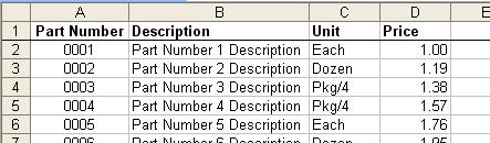
Double-click the sheet tab and give the worksheet a name. I called this one PriceList.
Make sure you formatted the Price column as numbers with 2 decimals (or currency, but I personally feel this just crowds the data).
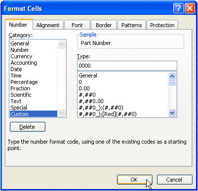
If you are following our directions here instead of using your own part numbers, you'll want to select Column A, and hit Format Cells, choose Custom format, and type in 0000, as shown. That means we can type our part numbers in with just 1, 2, 3...instead of typing all those zeroes.
Naming Ranges
Click on cell A2, and hit Shift+Ctrl then hit your down arrow one time. If you left no blank cells in column A (and you shouldn't have), then it'll select all your part numbers. From the menu, choose Insert Name Define and name it partnos, with no spaces. Hit OK.
Now click on Cell A2, and hit Shift+Ctrl+End. This should select all your data in the price list. Hit Insert Name Define and name it prices. Hit OK.
Our price list is now ready.
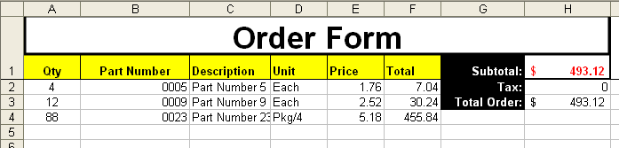
The Order Form
Drag Sheet2's tab to the left of the PriceList tab. Double-click it and rename it OrderForm.
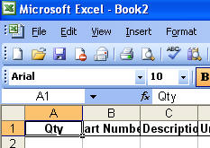
Copy the headings from your PriceList sheet over to your OrderForm sheet. Then select column A and insert a new column by hitting Insert Column. Type Qty into A1 to create a column in which to enter quantities.
Format the width of the columns to be wide enough for any entry from your PriceList.
Format the Part Number column the same way your part numbers are formatted on the PriceList worksheet. Format the Price and Total columns as numbers with 2 decimals. (You can use the format painter!)
Do the following:
- Click on Cell A2, and hit Window Freeze Panes. That way, no matter how many entries are made, the headings will remain at the top.
- Format the width of the columns to be wide enough for any entry from your PriceList.
- Format the Part Number column the same way your part numbers are formatted on the PriceList worksheet. Format the Price and Total columns as numbers with 2 decimals. (You can use the format painter!)
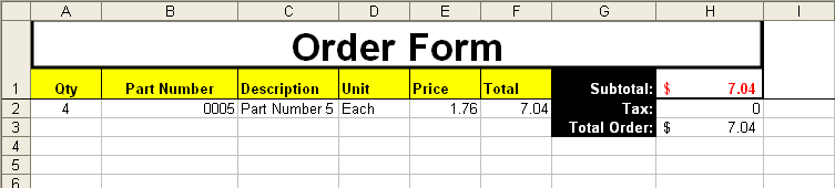
- In G1, type Subtotal
- In G2, type Tax
- In G3, type Total
- Create a textbox using the drawing toolbar. Put a title in it, make it the width of your cells.
- Make the height of row 1 tall enough so you can see the labels below the textbox.
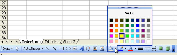
- Fill the heading and total cells with color using the Fill Bucket.
Data Validation Drop-Down
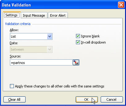
Select cells B2 to B200 (a quick way is to hit Edit Go to and type B2:B200, Enter). From the menu, choose Data Validation. Choose List from the drop-down and type: =partnos
Hit OK.
In cell C2, type the following formula:
=IF(ISBLANK(B2),"",VLOOKUP(B2,prices,2,FALSE))
For more information on the VLOOKUP formula, and how it works, click here.
Type the following formulas:
- In D2, type: =IF(ISBLANK(B2),"",VLOOKUP(B2,prices,3,FALSE))
- In E2, type: =IF(ISBLANK(B2),"",VLOOKUP(B2,prices,4,FALSE))
- In F2, type: =IF(OR(ISBLANK(A2),ISBLANK(B2)),"",A2*E2)
- In G2, type: =IF(SUM(F2:F200)=0,"",SUM(F2:F200))
- In G3, type: =IF(OR(ISBLANK(A2),ISBLANK(B2)),"",H1*I2)
- In G4, type: =SUM(H1:H2)
- In I2, type your tax rate, such as 6%
Select cells D2, through G2, and copy those formulas down to row 200.
Select row 201. Hit Shift+Ctrl plus your down arrow key, and then hit Format Row Hide. You can hide the unneeded columns, too.
Select cells A2 through B200 and hit Format Cells, choose the Protection tab, and unlock the cells. Go to Tools Protection, Protect Sheet and (add a password if you like and) hit OK.
Save the file.
Use the File
Type a quantity into cell A2, and choose a part number from the drop-down in B2. I have no tax percentage in cell I2, so the tax comes to zero.
Continue adding items in rows, and watch the values change for you automatically.