Access  ¨  Excel  ¨ FrontPage ¨ Outlook ¨ PowerPoint ¨  Word ¨    Miscellaneous  ¨  Tutorials  ¨  Windows  ¨  Free Downloads

Drop-Down Using Data Validation in Microsoft Excel

This article demonstrates how to create a drop-down list using either an absolute reference or a named range. When creating forms, you can force the user to choose one of the options, thus reducing errors.

If you need what is called "conditional" or "cascading" drop-downs, where the second dropdown is dependent upon the choice in the first drop-down, and so on, you may want to try this link.

Step 1. Create a list of options from which to choose.

Start by first creating a list of the drop-down choices you want to provide. Generally, when creating forms, you may need to provide more than one drop-down. If you create these on a separate worksheet, they are "out of the way" when your form is active. Because we use a separate worksheet, however, we must use a named range for our options list. It is not possible to use typical cell referencing when your option choices reside on another worksheet. Because of this, we recommend you always use a named range when creating this type of drop-down.

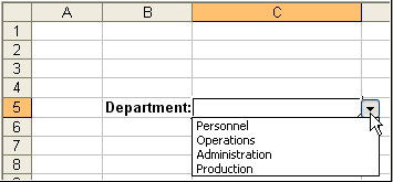
We chose department names for our example. You can list as many as you like, but don't leave any spaces. Our example contains the list of choices on a worksheet called "Data".

Tip. Make the first option in your list "Choose" or "Pick from List" to provide directions to the user of the form.

Step 2. Name the range that contains the options.

We then select our range of options, and assign a name to the range by typing it into the Name box (that drop-down just above column A in any worksheet), as shown below, and then hit Enter. Alternatively, you can select the options, and choose from the menus InsertàNameàDefine, and type the name there, and hit Enter.

Our sample has a named range called "depts".

Step 3. Assign validation to the cell.

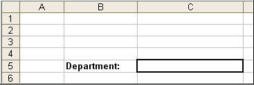
On our "front-end" worksheet—that is, the worksheet that contains the form, we provide a label for the drop-down in B5. We put a nice heavy border on cell C5. Then, select cell C5 and choose from the menu DataàValidation, and the Data Validation dialog appears. From the Allow: drop-down, we choose List, as shown below:

We then type an equal sign, followed by our range name, into the Source: box, as shown:

Tip. Don't forget the equal sign! If you do, the only option that will appear in your dropdown is the word that you typed!

Alternatively, if you have only several options from which to choose, and they're not likely to change, you can actually skip Step 1 and just type the list into the Source: box, separating each option with commas, as shown below. When typing text options directly into the Source: box, no equal sign is required.

Hit the OK button to apply the Data Validation to your cell. Click on the cell to activate it again, and a drop-down arrow appears next to your cell.

Step 4. Test to see that it worked.

Click the drop-down arrow to view your choices. Select one of the choices.

Check out the Input Message tab of the Data Validation dialog. Any Input Message you provide is displayed as a tool-tip when the cell is selected.

Tip. The arrow doesn't show unless the cell is selected. There is no way to alter it to show the arrow using the Data Validation method.

Use Conditional Formatting to format the cell to have a colored background if it is blank. This lets the user know that a choice is to be made.

Tip. Making the dropdown provide unique options from a list that contains the same options multiple times requires custom programming.

To "copy" the drop-down to other cells, use the Format Painter.

All contents copyright Anne Troy 2005-2006