Conditional Formatting with Formulas in Microsoft Excel
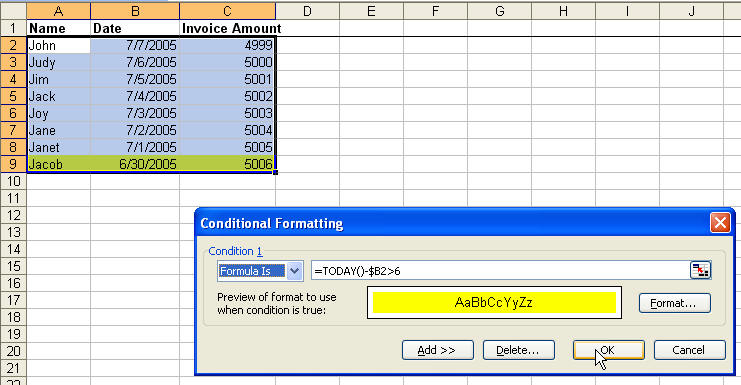
Sometimes, you need to just see something for it to work. In the following, we highlight all 3 cells of a record if the invoice date is older than 6 days (now one week old). I couldn't get this right the first time, and Jake Hilderband pointed out that I only needed a $ in front of the column reference, and not in front of the row reference. Don't ask me how, but the conditional formatting works a lot like autofilling a formula. You enter just the first one (here it's cell B2) and it automatically works on all of them (B3 through B9). If we remove the $ then it would be looking for dates in columns A and C as well-not good.
This article was actually requested by "Fraryl" via our. So, I'll provide the example that he/she did.
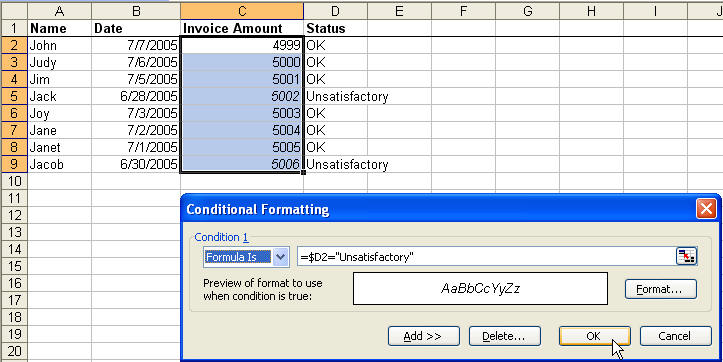
Example: If cell B3 has the word unsatisfactory, italicize the content in cell A3. Note how we put our text in quotes, as is done with most formulas. Admittedly, when I first did this, I also selected cell C1, and the italics formatting occurred in C4 and C8. Then I realized, I'd be looking first one cell down, and THEN to the right, which of course wasn't right.
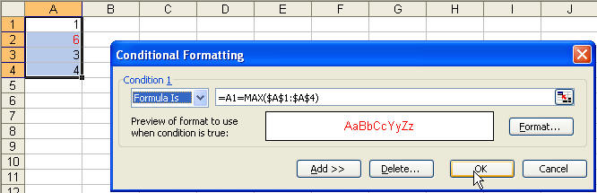
Example: Format as red font color the highest value in a range.